Gradient Descent Explained: How AI Adjusts Its Weights

In the first article in this series, we built a delivery-fee model from a distance, a weight and a bias. We could change those numbers by hand and see the prediction improve.

But a real training process needs a repeatable way to choose the changes. How much should a weight move? Should it increase or decrease?

Gradient descent uses the slope of a loss function to calculate parameter updates. We can follow one complete update with a calculator, then connect it to the training of larger neural networks. [1]

Start with a prediction that is too low

Our fictional delivery model has this form:

Predicted fee = distance × weight + bias

The earlier example used ₦200 per kilometre and a ₦500 base fee. That produced ₦1,700 for a 6 km journey.

For this demonstration, suppose our training data includes that same journey with a recorded fee of ₦1,700. Start with a poorer weight of ₦100 per kilometre. Keep the bias at ₦500 so we can focus on updating just one number.

To keep the arithmetic manageable, express money in units of ₦100. The target becomes 17, the weight becomes 1, and the bias becomes 5. Distance stays in kilometres.

Our prediction is therefore:

6 × 1 + 5 = 11

That means ₦1,100, which is ₦600 below the recorded fee. These are invented teaching figures, not current delivery prices.

Turn the error into a loss

We need a score for how far the prediction is from the target. For this example, use squared error:

Loss = (prediction − target)²

Our error is 11 − 17 = −6, so the loss is 36. Squaring makes errors in either direction positive and penalises larger errors more strongly. With several examples, we can average their squared errors to get mean squared error. [2]

The loss of 36 is an error score in squared ₦100 units. It is not a fee. Keeping the units consistent matters: changing the numerical scale also changes the gradients and can change which learning rates work well.

What does the gradient tell us?

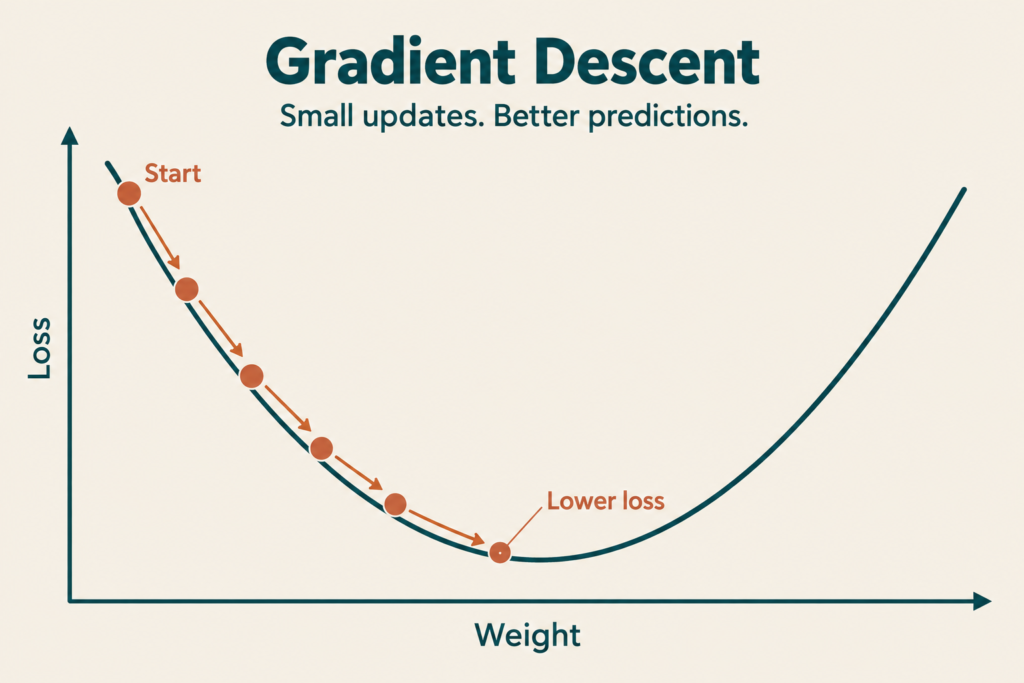
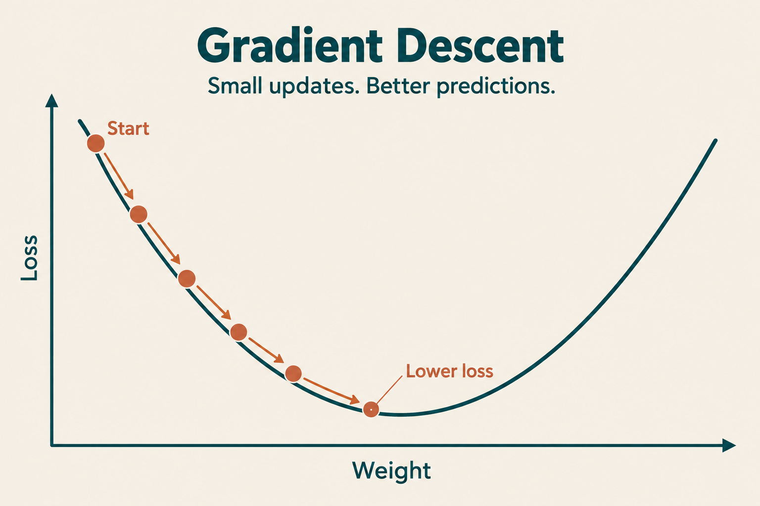
Imagine plotting the weight horizontally and the loss vertically. For our example, the graph is a bowl. Each point represents the loss at a particular weight, with everything else fixed.

At our starting weight, increasing the weight slightly lowers the loss. The slope is negative. On the other side of the bowl, increasing the weight raises the loss, so the slope is positive.

For one adjustable number, the gradient is this slope. It describes the local rate of change of loss. With several parameters, the gradient contains one such rate for each parameter. [3]

For our squared-error formula, the weight gradient is:

Weight gradient = 2 × (prediction − target) × distance

Substitute the numbers:

2 × (11 − 17) × 6 = −72

You do not need to derive that formula to follow the update. The factor of 2 comes from differentiating the square; the distance appears because changing the weight changes the prediction by distance times that change. The gradient is −72 at this particular starting point.

Make one gradient-descent update

The update rule is:

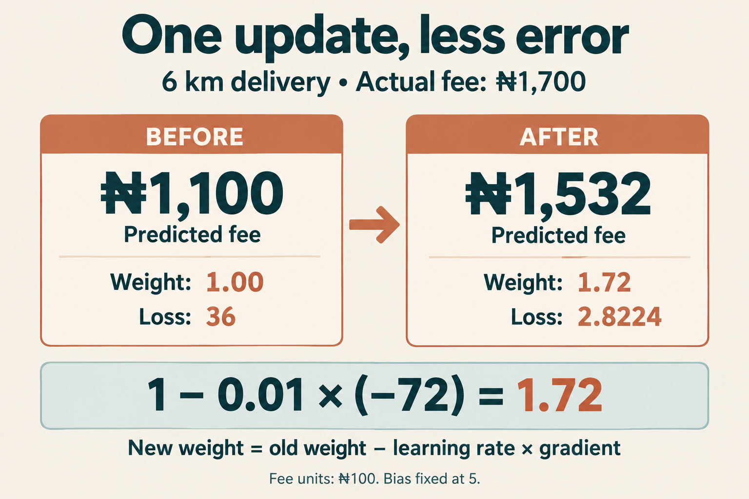
New weight = old weight − learning rate × weight gradient

The learning rate controls how much of the gradient we use in each update. Choose 0.01 for this example. This value is a teaching choice, not a universal recommendation. [4]

New weight = 1 − 0.01 × (−72) = 1.72

Subtracting a negative number increases the weight. In our original money units, it has moved from ₦100 to ₦172 per kilometre.

Now calculate a fresh prediction and loss:

Prediction: 6 × 1.72 + 5 = 15.32, or ₦1,532
Error: 15.32 − 17 = −1.68, or ₦168 too low
Loss: (−1.68)² = 2.8224

The loss has fallen from 36 to 2.8224. This update was calculated from the gradient rather than chosen by trial and error.

A worked update uses distance 6, target 17, fixed bias 5 and starting weight 1. The gradient is minus 72, the updated weight is 1.72 and the new prediction is 15.32. — Figure 2. With bias fixed at 5 and learning rate 0.01, one update changes the weight from 1 to 1.72 and reduces squared loss from 36 to 2.8224. Fees are in units of ₦100.

For the next update, recalculate the gradient using the new prediction:

New gradient = 2 × (15.32 − 17) × 6 = −20.16

Next weight = 1.72 − 0.01 × (−20.16) = 1.9216

The resulting prediction is 16.5296, or ₦1,652.96. The step has become smaller because the gradient has become smaller. Repeating this particular process moves the weight towards 2, equivalent to ₦200 per kilometre.

Why the learning rate matters

Return to the original weight of 1 and gradient of −72. Different learning rates produce different first steps:

0.001: the weight becomes 1.072 and the loss is about 31.00. Progress is relatively slow.
0.01: the weight becomes 1.72 and the loss is about 2.82. This step works well here.
0.03: the weight becomes 3.16 and the loss is about 48.44. The update overshoots and makes the prediction worse.

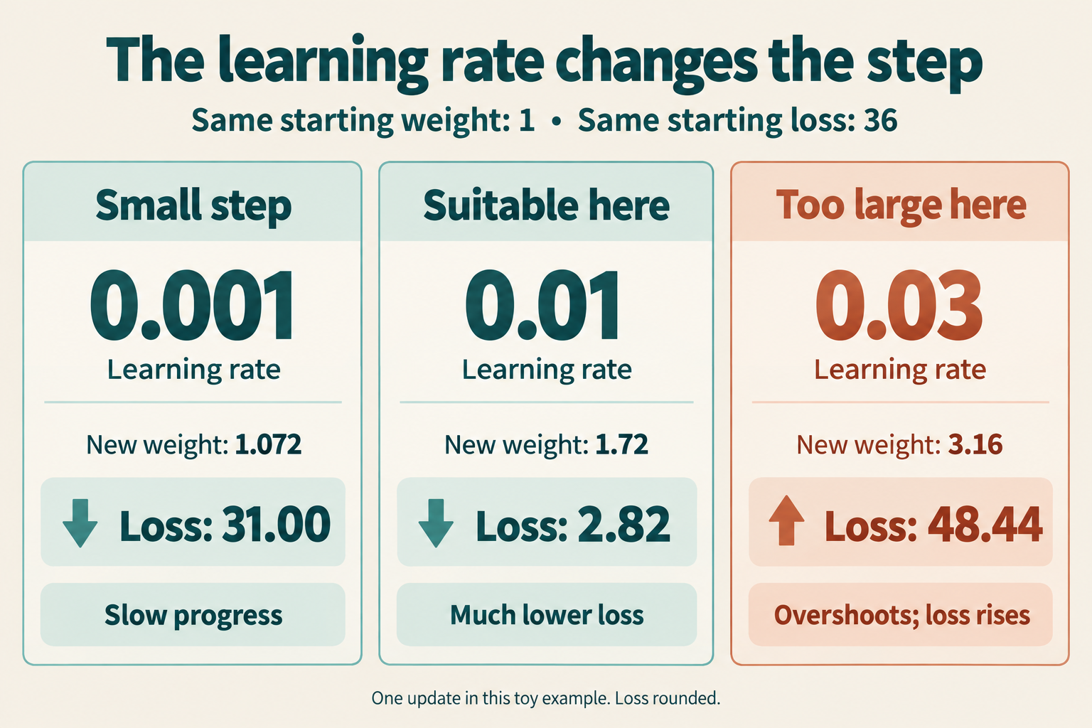
Three learning rates produce weights 1.072, 1.72 and 3.16, with losses approximately 31.00, 2.82 and 48.44. The largest update overshoots. — Figure 3. Starting from the same weight, learning rates 0.001, 0.01 and 0.03 yield different results. Losses are rounded; these values apply to this scaled example.

A very small learning rate can require many updates. A rate that is too large can cause oscillation or divergence. The right scale depends on the problem, and training systems may change the learning rate over time. [4]

The minus sign gives a locally downhill direction. It does not guarantee that a large jump will land at a lower point.

What happens to the bias and other weights?

We held the bias fixed to make the first calculation easier. Normally, a trainable bias gets its own gradient and update.

In our single-example model, the bias gradient is 2 × (prediction − target). At the original settings, that is −12. With learning rate 0.01, the bias would move from 5 to 5.12.

If we update both parameters, we calculate both gradients from the same pre-update settings. The new weight is 1.72 and the new bias is 5.12, giving a prediction of 15.44. That is a different experiment from the fixed-bias walkthrough above.

One recorded journey cannot uniquely determine both a per-kilometre charge and a base fee. Many combinations produce the same answer for 6 km. Records covering different distances provide information about both.

With many training examples, updates can use the whole dataset or a smaller mini-batch. A mini-batch makes each update cheaper, but its gradient may differ from the full-dataset gradient, so loss need not fall smoothly at every step. [4]

Where does backpropagation fit?

A neural network may contain many layers and millions of adjustable numbers. The training process still needs gradients for those numbers.

Backpropagation calculates the gradients efficiently through the network, working backwards through the operations used to produce the prediction. An optimizer uses those gradients to update parameters. Basic gradient descent is one update method; more elaborate optimizers modify how updates are formed. [5] [6]

Those are separate jobs within the same training loop: predict, measure loss, calculate gradients, update parameters, repeat.

Lower training loss is only part of the goal

Our one-weight example has a simple bowl-shaped loss. Large neural networks have much more complicated loss surfaces. Gradient-based training does not promise the best possible solution for every model and dataset.

Even a falling training loss does not prove that a model will perform well on unfamiliar inputs. Developers evaluate held-out data and watch for overfitting: improving on training examples while performing poorly on new ones. [7]

Finally, these updates happen during training. During ordinary inference, a trained model uses its existing parameters to produce a result. Generating an answer does not, by itself, mean its weights have changed. [8]

The useful idea to carry forward is simple: a prediction produces a measurable loss, gradients describe how that loss responds to parameter changes, and an update rule turns that information into new parameter values. Our move from ₦100 to ₦172 per kilometre is one small, fully visible example of that process.

Sources and further reading

The delivery examples and calculations are original teaching material. Technical explanations were checked against these primary references: